Pytorch Compiler Introduction

Summary

This article introduces the Compiler of PyTorch, starting with code examples to demonstrate the acceleration effects of compilation. Subsequently, basic knowledge related to PyTorch FX, and finally, contents about TorchDynamo is presented, including Graph, adjustments to Python bytecode, Guard, Cache, etc.

Preamble: This document is based on Pytorch 2.1, TorchDynamo is a continuously iterating module, later versions may have different API, but the core idea remains the same.

Overview

torch.compile is a feature introduced in Pytorch2.x for more accurately capturing the computation graph and accelerating program execution. It is written in Python, marking a gradual shift in Pytorch development from C++ to Python.

torch.compile mainly relies on the following technologies:

• TorchDynamo (torch._dynamo): An internal API, using CPython’s Frame Evaluation API to safely capture PyTorch computation graphs.
• TorchInductor: The default torch.compile deep learning compiler, generating efficiently executable code for various backends. For NVIDIA and AMD GPUs, it’s primarily built on OpenAI Triton.
• AOT Autograd (Ahead-Of-Time Autograd): Captures user-level code and backpropagation at compile-time. Generally, deep learning frameworks execute forward and backward operations at runtime, while AOT Autograd allows capturing backpropagation at compile-time, then using TorchInductor to accelerate forward computation and backpropagation.

Some common backends include:

• Support for both training and inference:
  • inductor: The default TorchInductor backend.
  • cudagraphs: A Cuda computation graph backend with AOT Autograd.
  • ipex: intel-extension-for-Pytorch, a CPU backend.
  • onnxrt: Training backend based on ONNX Runtime, CPU / GPU.
• Support for inference:
  • tensorrt: onnx-tensorrt, using ONNX Runtime to run TensorRT for accelerated inference.
  • tvm: Using Apache TVM for accelerated inference.

Getting Started

 1
 2
 3
 4
 5
 6
 7
 8
 9
10
11
12
13
14
15
16
17
18
19
20
21
22
23
24
25
26
27
28
29
30
31
32
33
34

import torch
import time

def fn(x):
    a = torch.cos(x)
    b = torch.sin(a)
    return b

new_fn = torch.compile(fn, backend="inductor")

input_tensor = torch.randn([1024, 1024, 1024]).to(device="cuda:0")

start_time = time.time()
_ = fn(input_tensor)
torch.cuda.synchronize()    # syncronize
original_duration = (time.time() - start_time)

start_time = time.time()
_ = new_fn(input_tensor)
torch.cuda.synchronize()
compiled_duration = (time.time() - start_time)

start_time = time.time()
_ = new_fn(input_tensor)
torch.cuda.synchronize()
compiled_duration2 = (time.time() - start_time)

print(f"Original duration  : {original_duration:.6f} seconds")
print(f"Compiled duration  : {compiled_duration:.6f} seconds")
print(f"Compiled duration 2: {compiled_duration2:.6f} seconds")

# Original duration  : 0.025237 seconds
# Compiled duration  : 4.118577 seconds
# Compiled duration 2: 0.010665 seconds

In the code above, we compared the runtime of the original function with the compiled function, and we can see that, after the initial overhead (extra initialization or compilation time required for the first call), our function has been accelerated by more than twice, which is very beneficial in actual training scenarios where multiple repetitions are needed.

There are mainly two reasons for the acceleration, firstly, we achieved fusion through compile.

What is fusion? TorchInductor supports Triton kernel by default, and we can observe the generated Triton code by setting the environment variable TORCH_COMPILE_DEBUG=1 (code may vary with different hardware).

 1
 2
 3
 4
 5
 6
 7
 8
 9
10
11
12

@pointwise(size_hints=[1073741824], filename=__file__, meta={'signature': {0: '*fp32', 1: '*fp32', 2: 'i32'}, 'device': 0, 'constants': {}, 'mutated_arg_names': [], 'configs': [instance_descriptor(divisible_by_16=(0, 1, 2), equal_to_1=())]})
@triton.jit
def triton_(in_ptr0, out_ptr0, xnumel, XBLOCK : tl.constexpr):
    xnumel = 1073741824
    xoffset = tl.program_id(0) * XBLOCK
    xindex = xoffset + tl.arange(0, XBLOCK)[:]
    xmask = xindex < xnumel
    x0 = xindex
    tmp0 = tl.load(in_ptr0 + (x0), xmask)
    tmp1 = tl.cos(tmp0) # stored in registers that are very efficient
    tmp2 = tl.sin(tmp1)
    tl.store(out_ptr0 + (x0 + tl.zeros([XBLOCK], tl.int32)), tmp2, xmask)

In the original function, for pointwise operations like cos and sin, x needs to be read once, computed and written into a, then a is read again, computed and written into b. Now through fusion, we have only performed one read using tl.load to tmp0, and one write using tl.store. We know that in newer GPUs, the bottleneck lies in memory bandwidth (speed when accesses data) rather than computation (floating point operation speed), hence fusion provides a good performance optimization.

Secondly, inductor also provides support for Cuda graphs. Cuda graphs capture a sequence of operations (such as kernel calls, memory copies, etc.) and save it as a graph. Based on this graph, the same sequence of operations can be executed multiple times, significantly reducing the overhead of launching operations. NVIDIA might also optimize the graph to reduce synchronization or improve memory access patterns, further increasing efficiency.

FX

FX, standing for PyTorch Flexible eXtensions, is something we need to understand before diving into Dynamo.

FX is a sub-library of Pytorch, designed to assist developers in transforming nn.Module model instances into IR (Intermediate Representation). IR is a more structured and analyzable graph.

Developers can perform visual analysis, model transformation, and optimization (such as removing unnecessary operations, merging layers, etc.) based on IR. Once optimized, it can be converted back into Pytorch code or other formats through code generation, facilitating deployment to different platforms and backends.

FX primarily comprises three components: symbolic tracer, IR, and Python code generation. Let’s elucidate these three components with an example:

 1
 2
 3
 4
 5
 6
 7
 8
 9
10
11
12
13
14
15
16
17
18
19
20
21

import torch
class MyModule(torch.nn.Module):
    def __init__(self):
        super().__init__()
        self.param = torch.nn.Parameter(torch.rand(3, 4))
        self.linear = torch.nn.Linear(4, 5)

    def forward(self, x):
        return self.linear(x + self.param).clamp(min=0.0, max=1.0)

module = MyModule()

from torch.fx import symbolic_trace
# Invoking symbolic tracing to capture model semantics
symbolic_traced : torch.fx.GraphModule = symbolic_trace(module)

# print IR
print(symbolic_traced.graph)

# Python code generation
print(symbolic_traced.code)

Symbolic Tracer inputs some fake values (also known as Proxies) to the model, and the operations on these proxies are recorded.

IR (Intermediate Representation) is a container that records operations during symbolic tracing, containing inputs, call sites (functions/methods/nn.Module instances), and return values. For instance, the above code will generate the following IR:

1
2
3
4
5
6
7
8
9

"""
graph():
    %x : [num_users=1] = placeholder[target=x]
    %param : [num_users=1] = get_attr[target=param]
    %add : [num_users=1] = call_function[target=operator.add](args = (%x, %param), kwargs = {})
    %linear : [num_users=1] = call_module[target=linear](args = (%add,), kwargs = {})
    %clamp : [num_users=1] = call_method[target=clamp](args = (%linear,), kwargs = {min: 0.0, max: 1.0})
    return clamp
"""

Python Code Generation can help us create effective Python code that matches the semantics based on IR, as the example above would generate the following Python code:

1
2
3
4
5
6

def forward(self, x):
    param = self.param
    add = x + param;  x = param = None
    linear = self.linear(add);  add = None
    clamp = linear.clamp(min = 0.0, max = 1.0);  linear = None
    return clamp

These three components can be used in combination or separately (like using symbolic tracing alone for model analysis), serving as handy tools for developers.

Deep Dive to TorchDynamo

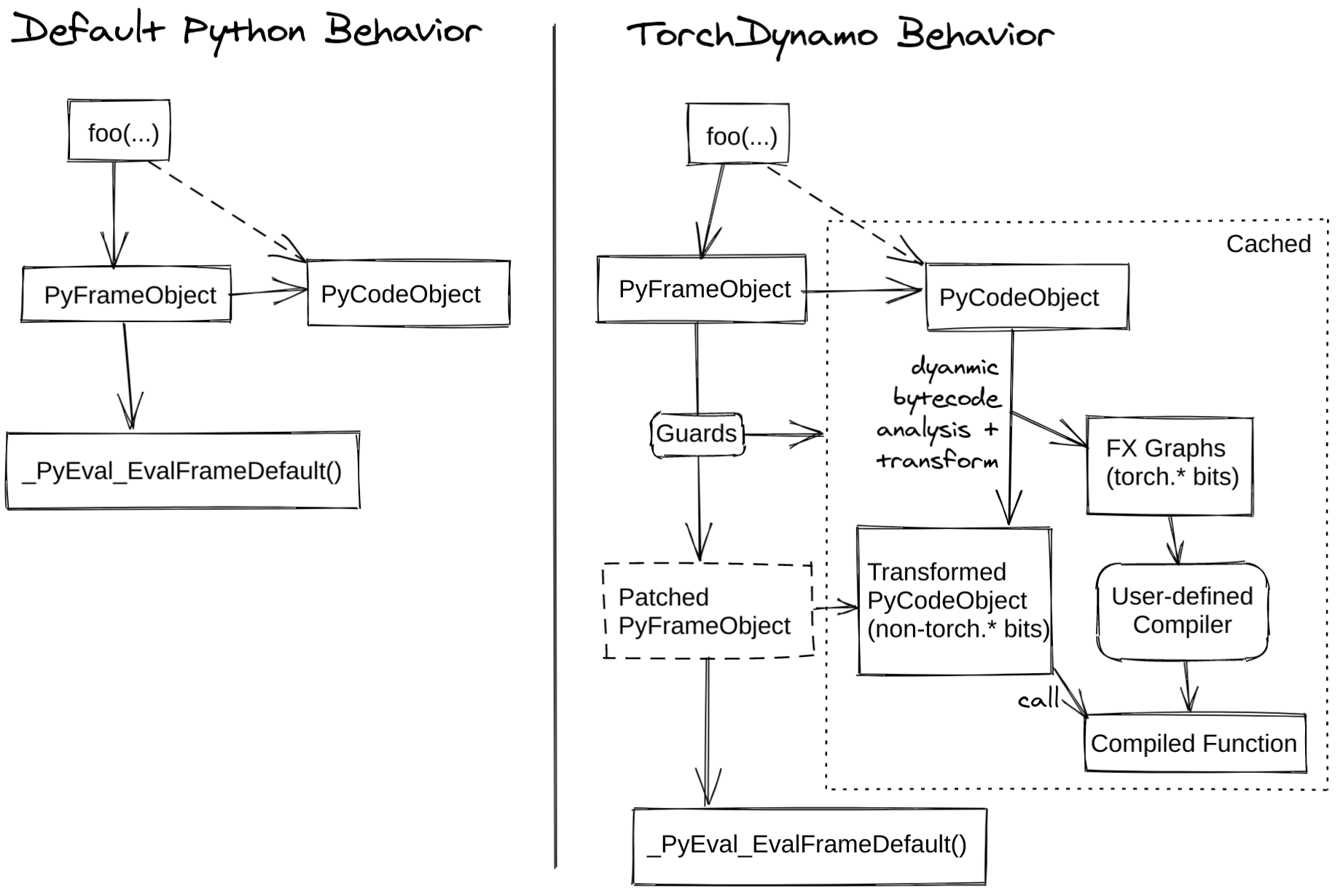
TorchDynamo is a Python-level JIT (just-in-time) compiler, utilizing CPython’s Frame Evaluation API (PEP523) to rewrite Python bytecode and extract Pytorch operation sequences and form an FX Graph, which is then compiled using a specified backend. By creating FX Graph through bytecode analysis, and combining Python execution with the compiled backend, we ensure usability while maintaining good performance.

The image below explains the mechanism of torch.compile:

Example

 1
 2
 3
 4
 5
 6
 7
 8
 9
10
11
12
13
14
15
16
17
18

from typing import List
import torch
from torch import _dynamo as torchdynamo


def my_compiler(gm: torch.fx.GraphModule, example_inputs: List[torch.Tensor]):
    print("my_compiler() called with FX graph:")
    gm.graph.print_tabular()
    return gm.forward  # returns Python callable object

@torchdynamo.optimize(my_compiler)
def toy_example(a, b):
    x = a / (torch.abs(a) + 1)
    if b.sum() < 0:
        b = b * -1
    return x * b
for _ in range(100):
    toy_example(torch.randn(10), torch.randn(10))

Executing the above code, we can get:

 1
 2
 3
 4
 5
 6
 7
 8
 9
10
11
12
13
14
15
16
17
18
19
20
21
22
23
24
25
26
27
28

my_compiler() called with FX graph:
opcode         name     target                              args               kwargs
-------------  -------  -----------------------------  ---------------------  --------
placeholder    a        a                                    ()                 {}
placeholder    b        b                                    ()                 {}
call_function  abs_1    <built-in method abs>                (a,)               {}
call_function  add      <built-in function add>              (abs_1, 1)         {}
call_function  truediv  <built-in function truediv>          (a, add)           {}
call_method    sum_1    sum                                  (b,)               {}
call_function  lt       <built-in function lt>               (sum_1, 0)         {}
output         output   output                               ((truediv, lt),)   {}

my_compiler() called with FX graph:
opcode         name    target                   args         kwargs
-------------  ------  -----------------------  -----------  --------
placeholder    b       b                        ()           {}
placeholder    x       x                        ()           {}
call_function  mul     <built-in function mul>  (b, -1)      {}
call_function  mul_1   <built-in function mul>  (x, mul)     {}
output         output  output                   ((mul_1,),)  {}

my_compiler() called with FX graph:
opcode         name    target                   args       kwargs
-------------  ------  -----------------------  ---------  --------
placeholder    b       b                        ()         {}
placeholder    x       x                        ()         {}
call_function  mul     <built-in function mul>  (x, b)     {}
output         output  output                   ((mul,),)  {}

This output informs us that my_compiler was called three times, generating three graphs:

1. All content before the branch: Compute x and check if b.sum() is less than 0.
2. The True branch of if: Includes b = b * -1 and return x * b.
3. The False branch of if: Just the return value return x * b.

What does Dynamo do?

To delve deeper into what Dynamo specifically does in the process above, we can add the following code to print more logs:

1
2
3
4
5

import torch._dynamo.config
import logging

torch._dynamo.config.log_level = logging.INFO
torch._dynamo.config.output_code = True

The output of the first graph is as follows:

 1
 2
 3
 4
 5
 6
 7
 8
 9
10
11
12
13
14
15
16
17
18
19
20
21
22
23
24
25
26
27
28
29
30
31
32
33
34
35
36
37
38
39
40
41
42
43
44
45
46
47
48
49
50
51
52
53
54
55
56
57
58
59
60

torch._dynamo.symbolic_convert: [INFO] Step 1: torchdynamo start tracing toy_example
torch._dynamo.output_graph: [INFO] Step 2: calling compiler function my_compiler
torch._dynamo.output_graph: [INFO] Step 2: done compiler function my_compiler
torch._dynamo.output_graph: [INFO] TRACED GRAPH 

# ... graph printed before

torch._dynamo.convert_Frame: [INFO] ORIGINAL BYTECODE toy_example test_graph.py line 17 
 19           0 LOAD_FAST                0 (a)
              2 LOAD_GLOBAL              0 (torch)
              4 LOAD_METHOD              1 (abs)
              6 LOAD_FAST                0 (a)
              8 CALL_METHOD              1
             10 LOAD_CONST               1 (1)
             12 BINARY_ADD
             14 BINARY_TRUE_DIVIDE
             16 STORE_FAST               2 (x)

 20          18 LOAD_FAST                1 (b)
             20 LOAD_METHOD              2 (sum)
             22 CALL_METHOD              0
             24 LOAD_CONST               2 (0)
             26 COMPARE_OP               0 (<)
             28 POP_JUMP_IF_FALSE       38

 21          30 LOAD_FAST                1 (b)
             32 LOAD_CONST               3 (-1)
             34 BINARY_MULTIPLY
             36 STORE_FAST               1 (b)

 22     >>   38 LOAD_FAST                2 (x)
             40 LOAD_FAST                1 (b)
             42 BINARY_MULTIPLY
             44 RETURN_VALUE

 
torch._dynamo.convert_Frame: [INFO] MODIFIED BYTECODE toy_example test_graph.py line 17 
 17           0 LOAD_GLOBAL              3 (__compiled_fn_0)
              2 LOAD_FAST                0 (a)
              4 LOAD_FAST                1 (b)
              6 CALL_FUNCTION            2
              8 UNPACK_SEQUENCE          2
             10 STORE_FAST               2 (x)
             12 POP_JUMP_IF_FALSE       24
             14 LOAD_GLOBAL              4 (__resume_at_30_1)
             16 LOAD_FAST                1 (b)
             18 LOAD_FAST                2 (x)
             20 CALL_FUNCTION            2
             22 RETURN_VALUE
        >>   24 LOAD_GLOBAL              5 (__resume_at_38_2)
             26 LOAD_FAST                1 (b)
             28 LOAD_FAST                2 (x)
             30 CALL_FUNCTION            2
             32 RETURN_VALUE

 
torch._dynamo.convert_Frame: [INFO] GUARDS:
 - local 'a' TENSOR_MATCH # ... 
 - local 'b' TENSOR_MATCH # ...   
 - global 'torch' FUNCTION_MATCH # ...

From the output, it’s clear that Dynamo starts by tracing our function toy_example, then compiles, generates the graph, and outputs it. Additionally, the output reveals changes in bytecode and the declaration of Guards.

Let’s first look at the bytecode:

In the original Python bytecode, operations like LOAD_FAST are used to load values from local variables, LOAD_METHOD and CALL_METHOD are used to call methods, BINARY_ADD and BINARY_MULTIPLY are used for addition and multiplication operations, respectively.

Dynamo modifies the Python bytecode, replacing the calculations for x and the check for b.sum() < 0 in the original bytecode with a call to the compiled __compiled_fn_0 function. Subsequently, based on the returned value, it calls the generated __resume_at_30_1 or __resume_at_38_2, corresponding to the two branches in the original bytecode.

__resume_at_xx functions come from the following template, and are used to continue executing code in the graph at the breakpoint.

1
2
3
4

__resume_at_<offset>:
    ... restore stack state if needed ...
    JUMP_ABSOLUTE <offset> into toy_example
    ... original bytecode of toy_example ...

By generating __resume_at_xx, we force the function to execute in a new Python Frame, and recursively initiate Dynamo to execute the capture process again.

How to understand this recursion? When toy_example is executed for the first time, Dynamo initiates a capture process, generating optimized bytecode, including __compiled_fn_0 and two resume functions. When we enter a resume function, Dynamo initiates a similar process to handle other possible branches within the resume function, and so on, processing all the code.

Guard

The output above also includes Guard:

1
2
3
4

torch._dynamo.convert_Frame: [INFO] GUARDS:
 - local 'a' TENSOR_MATCH # ... 
 - local 'b' TENSOR_MATCH # ...   
 - global 'torch' FUNCTION_MATCH # ...

Here, if any Guard fails (meaning the optimized code is not safe or correct, or possibly failing due to different runtime conditions), the graph will be re-captured and re-compiled.

In this case, TENSOR_MATCH checks tensor object attributes like dtype, shape, device, requires_grad, dispatch_key, ndim, sizes, strides, etc. FUNCTION_MATCH checks the function object’s id(obj), and possibly id(type(obj)) etc., to ensure correct function calls.

Caching

An important factor for acceleration in the above example by Dynamo is Caching. While Caching is not a direct accelerator, it prevents re-compilation.

After modifying the Python bytecode, Dynamo caches it. Every time a new Frame is received for evaluation, Dynamo checks if objects referenced in the Frame have changed; if not, the cached user bytecode is directly used.

The process can be summarized as follows:

1. Dynamo receives a Python Frame, which contains the current state and context information of the code.
2. Dynamo optimizes the Python instructions, generating optimized bytecode.
3. For the objects captured in (2), Dynamo creates tracking objects:
   1. tracking on an output graph (an internal implementation of torch.fx.Tracer)
   2. Guard.
4. Dynamo generates a check_fn function, which is used to check these Guard objects.
5. When the program runs into the associated code, check_fn is called to check the bytecode in the Cache. If check_fn returns True, it is used directly; otherwise, optimized code is regenerated through re-compilation or Graph Break.

Referrence

• TORCH.COMPILER
• GETTING STARTED
• Triton
• TORCHDYNAMO DEEP DIVE